Demystifying snGradScheme in OpenFOAM

What happens when you type gradSchemes { default corrected; }? While it seems like a simple keyword, you are selecting a powerful, pluggable piece of C++ code that dictates how gradients are calculated across the entire mesh. This choice has profound implications for the accuracy, stability, and performance of your simulation.

Today, we'll pull back the curtain on the snGradScheme framework. We'll explore how it works, what the common schemes actually do, and see exactly where they impact the matrices and source terms in your simulation's equations.

What is `snGrad`?

First, the name. snGrad stands for Surface-Normal Gradient. In the Finite Volume Method (FVM), we discretize equations over control volumes (cells). To evaluate a term containing a gradient, like the diffusion term ∇ ⋅ (Γ ∇φ), we use Gauss's theorem to convert the volume integral into a sum of fluxes over the cell's faces:

\[ \int_V \nabla \cdot (\Gamma \nabla\phi) \, dV = \sum_f \int_{S_f} (\Gamma \nabla\phi) \cdot d\mathbf{S} \approx \sum_f \Gamma_f (\nabla\phi)_f \cdot \mathbf{S}_f \]

The crucial term here is (∇φ)_f ⋅ S_f, which represents the flux of the gradient across a face. This requires calculating the component of the gradient ∇φ that is normal to the face f. This is the job of the snGrad schemes.

Explicit vs. Implicit: The Two Roles of `snGrad`

A common misconception is that gradSchemes are only used for explicit calculations, like when you want to visualize the pressure gradient. While that is one use, their more critical role is in the implicit discretization of differential operators.

Namespace	Treatment	How `snGrad` is Used	Result
`fvc::grad(p)`	Explicit	Directly called to compute the gradient field from known values.	A `volField` (a field of data).
`fvm::laplacian(nu, U)`	Implicit	Its underlying logic and coefficients are used to build the `A` matrix and `b` source vector in `Ax=b`.	An `fvMatrix` (a system of equations).

When you write fvm::laplacian(nu, U), OpenFOAM uses your chosen snGrad scheme to determine how the unknown field U in one cell implicitly affects its neighbors. This relationship is what forms the coefficients of the linear system that gets solved at every time step.

A Deep Dive: `orthogonal`, `uncorrected`, and `corrected`

To understand how these schemes work, let's visualize a non-orthogonal face between two cells, an "owner" (P) and a "neighbour" (N).

Non-Orthogonal Face Diagram

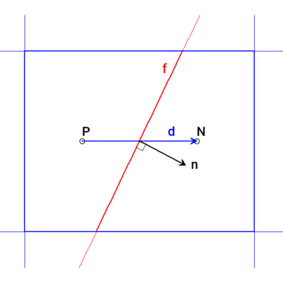
$d$: The vector connecting the cell centers (from P to N).
$n$ : The surface area vector of the shared face. It is always normal to the face.

In a non-orthogonal mesh, d is not parallel to n. This misalignment is the source of numerical error that schemes must handle.

1. `orthogonal`

This is the simplest, fastest, and most inaccurate scheme for real-world meshes. It operates on a bold assumption: it pretends the mesh is perfectly orthogonal.

Concept: It assumes the cell-center vector d is perfectly aligned with the face normal S_f.
Equation: The surface-normal gradient is approximated as: $$ (\nabla\phi)_f \cdot \mathbf{S}_f \approx \frac{|\mathbf{S}_f|}{ |\mathbf{d}|} (\phi_N - \phi_P) $$
Code: It achieves this by using the most basic geometric coefficients from the mesh.

  // In src/finiteVolume/finiteVolume/snGradSchemes/orthogonalSnGrad/orthogonalSnGrad.H
  virtual tmp<surfaceScalarField> deltaCoeffs(const VolField<Type>&) const
  {
      return this->mesh().deltaCoeffs();
  }

2. `uncorrected`

This scheme is smarter. It acknowledges that the mesh is non-orthogonal but chooses not to apply an explicit correction for it.

Concept: It correctly calculates the component of the cell-center vector d that is normal to the face. It uses the true projection but ignores the component of the gradient that arises from the misalignment.
Equation: The approximation uses the dot product to find the correct projection distance. $$ (\nabla\phi)_f \cdot \mathbf{S}_f \approx \frac{|\mathbf{S}_f|^2}{\mathbf{d} \cdot \mathbf{S}_f} (\phi_N - \phi_P) $$ The term d ⋅ S_f correctly accounts for the angle between the cell-center vector and the face normal.
Code: It uses the nonOrthDeltaCoeffs, which contain these more accurate geometric factors.

  // In src/finiteVolume/finiteVolume/snGradSchemes/uncorrectedSnGrad/uncorrectedSnGrad.H
  virtual tmp<surfaceScalarField> deltaCoeffs(const VolField<Type>&) const
  {
      return this->mesh().nonOrthDeltaCoeffs();
  }

3. `corrected`

This is the workhorse for most general-purpose CFD. It provides the full picture by taking the accurate orthogonal approximation from uncorrected and adding an explicit term to account for the non-orthogonality.

Concept: The gradient at the face is decomposed into an implicit orthogonal part and an explicit non-orthogonal correction.

\[ (\nabla\phi)_f \cdot \mathbf{S}_f = \underbrace{\frac{|\mathbf{S}_f|^2}{\mathbf{d} \cdot \mathbf{S}_f} (\phi_N - \phi_P)}_{ \text{Implicit Part}} + \underbrace{ \left( (\nabla\phi)_f - \frac{\mathbf{d}}{|\mathbf{d}|^2}(\phi_N - \phi_P) \right) \cdot \mathbf{S}_f}_{ \text{Explicit Correction}} \]

This separation into an implicit part and an explicit correction is the key to how it's implemented in the code.

The Laplacian Scheme: Where the Matrix is Built

We've seen that the snGradScheme provides the rules for the calculation, but where is the matrix actually assembled? This happens inside the chosen laplacianScheme. The default, Gauss, is the most common.

The gaussLaplacianScheme acts as the "builder." It takes the diffusivity (e.g., nu), looks up your chosen snGradScheme from fvSchemes, and uses it to construct the fvMatrix (the A matrix and b source vector).

Here is a simplified view of the code that performs this magic, found in src/finiteVolume/finiteVolume/laplacianSchemes/gaussLaplacianScheme/gaussLaplacianScheme.C:

  // Simplified from gaussLaplacianScheme.C

  // The 'fvmLaplacian' function is called when you write fvm::laplacian(...)
  template<class Type, class GType>
  tmp<fvMatrix<Type>>
  Foam::gaussLaplacianScheme<Type, GType>::fvmLaplacian
  (
      const GeometricField<Type, fvPatchField, volMesh>& vf,
      const GeometricField<GType, fvsPatchField, surfaceMesh>& gamma
  )
  {
      // ... (Matrix setup) ...

      // 1. Get the geometric coefficients from the chosen snGrad scheme (e.g., corrected)
      const surfaceScalarField& deltaCoeffs = snGradScheme_().deltaCoeffs(vf);

      // 2. IMPLICIT PART: Build the matrix coefficients (off-diagonals of A)
      //    gamma is the diffusivity (e.g., nu)
      //    This term becomes the coefficient for the neighbour cell in the owner cell's equation.
      internalCoeffs = gamma.internalField() * deltaCoeffs;

      // ... (Boundary condition handling) ...

      // 3. EXPLICIT PART: If the scheme is "corrected", add the correction to the source vector (b)
      if (snGradScheme_().corrected())
      {
          // This calls the correction() function on the correctedSnGrad object
          const tmp<SurfaceField<Type>> tfaceCorr = snGradScheme_().correction(vf);

          // The correction is added to the SOURCE TERM (b), not the matrix (A)
          // This makes the correction explicit, as it's based on values from the previous iteration.
          forAll(owner, facei)
          {
              source[owner[facei]]     -= tfaceCorr.ref()[facei];
              source[neighbour[facei]] += tfaceCorr.ref()[facei];
          }
      }
      // ... (Final matrix assembly) ...
  }

This code beautifully illustrates the separation of concerns:

The implicit part of the gradient (deltaCoeffs) is multiplied by the diffusivity and used to build the main and off-diagonal coefficients of the A matrix. This part is numerically stable and connects the unknown vf values between adjacent cells.
The explicit part (correction()) is calculated using known field values and is added to the source vector b. This ensures that even complex corrections don't destabilize the matrix, at the cost of being one time-step "behind."

A Quick Look at Other Schemes

While the three schemes above are the most fundamental, OpenFOAM provides others for specific needs:

limited: A wrapper scheme used to improve stability. It limits the magnitude of the non-orthogonal correction from a sub-scheme (e.g., limited corrected 0.5;).
linearFit & quadraticFit: Higher-order schemes that fit a polynomial to cell values around a face to compute a more accurate gradient. They are more computationally expensive.
faceCorrected: An alternative to the standard corrected scheme that uses interpolation to the face vertices, which can be more robust on highly skewed meshes.

Conclusion

The snGradScheme framework in OpenFOAM is a cornerstone of its numerical engine. Your choice in fvSchemes is not just a keyword; it's a selection of a specific numerical strategy that defines:

The geometric coefficients used for the primary gradient calculation.
Whether an explicit non-orthogonal correction is added.
How the implicit matrix and explicit source terms are constructed for operators like fvm::laplacian.

Understanding the difference between orthogonal, uncorrected, and corrected empowers you to make more informed decisions, leading to more accurate and stable simulations. The next time you set up a case, you'll know exactly what's happening under the hood.

Demystifying snGradScheme in OpenFOAM

What is snGrad?

Explicit vs. Implicit: The Two Roles of snGrad

A Deep Dive: orthogonal, uncorrected, and corrected

1. orthogonal

2. uncorrected

3. corrected